Explainability in Neural Networks, Part 4: Path Methods for Feature Attribution

Training neural networks involves gradients and differentiation, and it turns out that one good way of explaining a neural network's behavior (in terms of its inputs) is by integrating gradients...

In the last post we formalized several desirable properties of feature-attribution methods as Axioms of Attribution, and the post concluded by saying Path Integrated Gradient Methods (or Path Methods in short) satisfy many of these axioms. This post will delve deeper into these methods. We continue to use the formulation from the ICML 2017 paper by Sundararajan et. al.^[1] The detailed derivation is our own, and assumes the reader has some familiarity with differential and integral calculus.

Attribution along extremal paths is easy

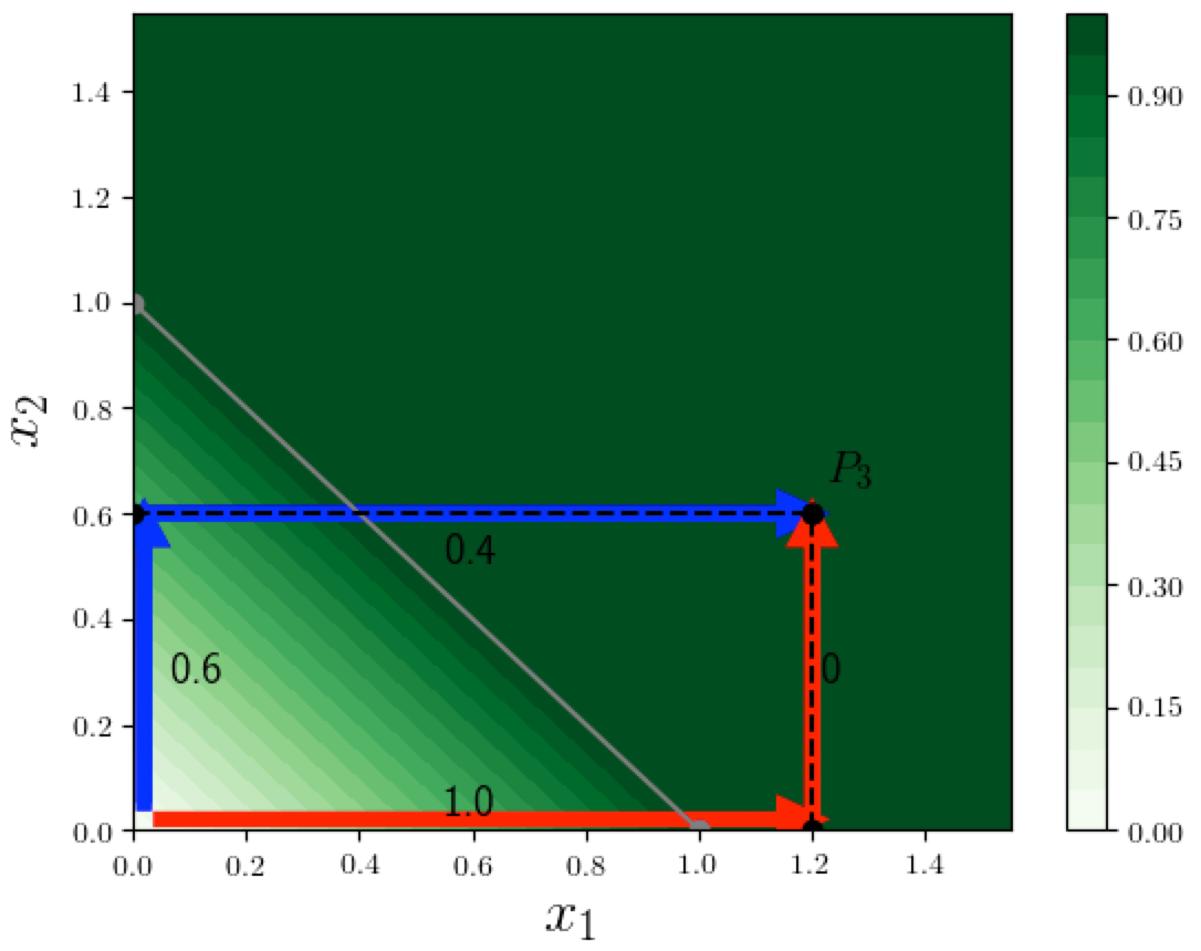
To understand the math behind Path Methods, it helps to recall our 2-dimensional example where the function computed by the neural network is $F(x) = \min(1, x_1 + x_2)$ (we will use this example in the rest of this post). Suppose we want to find the feature-attributions for the function value at point $P_3 = (1.2, 0.6)$. In the contour plot below we see two specific paths from the origin to $P_3$. Notice that these paths sequentially change one variable from 0 (the baseline value) to its final value at $P_3$: the red path changes $x_1$ first, then $x_2$. The blue path changes $x_2$ first, then $x_1$. There are of course an infinite number of possible paths from the origin to $P_3$, and paths such as these that sequentially change one variable at a time are called extremal paths (we informally called them "axis-parallel" paths in the last post). If the input $x$ is $d$-dimensional, there are $d!$ possible orderings of the input dimensions, and there would be $d!$ different extremal paths.

What is nice about extremal paths is that we can easily compute the contribution of each variable along a specific path. In the above example, when moving from the origin toward $P_3$ along the blue path, on the first segment only $x_2$ changes (from 0 to its final value 0.6), and causes $F$ to increase by $0.6$, and on the second segment only $x_1$ changes, and causes $F$ to increase by $0.4$, which results in attributions $(0.4, 0.6)$.

The reason it is simple to compute the contributions of each feature on an extremal path is that on each straight-line segment, only one feature changes. So this idea extends naturally to compute the feature-contributions along any step-like portion of a path, and we will see below how this is useful.

Parametric representation of general paths

Before moving on to discuss attribution along arbitrary paths, we should first consider how a general path can be represented. It is convenient to use a parametric representation of a path from the origin to $x$. Imagine we are moving along this path from the origin to $x$, and we introduce a parameter $\alpha$, which we will call the path position parameter, that represents the fraction of the path covered so far: this $\alpha$ uniquely identifies a point along the path. Then the path can be represented by a function $g$ that maps $\alpha$ to the $d$-dimensional coordinates of the unique point on the path that corresponds to $\alpha$.

Thus $g(\alpha)$ represents the $d$-dimensional coordinates of the point on the path at position $\alpha$. In particular $g(0)$ is the origin (all zero coordinates), and $g(1) = x$. We write $g_i(\alpha)$ to denote the $i$'th coordinate of $g(\alpha)$. We will only consider smooth functions $g$, i.e. those that are differentiable.

Attribution on general paths by step-approximation

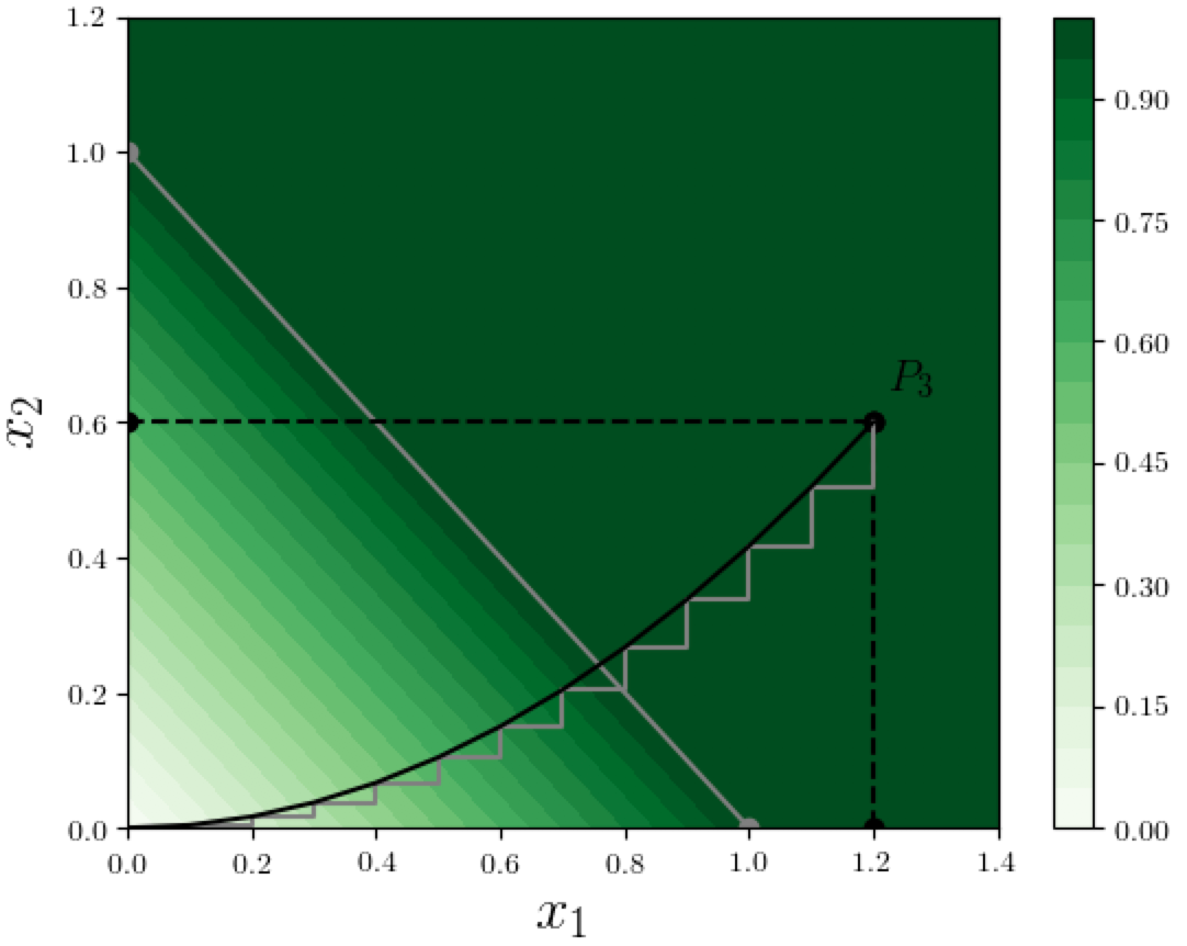
So how can we do attribution along an arbitrary path $\Pi$ from the origin to $P_3$? Here's a simple idea:

Since we already know how to do attribution along any "step-like" path, we approximate the path $\Pi$ with a sequence of infinitesimally small steps, as shown in the figure below.

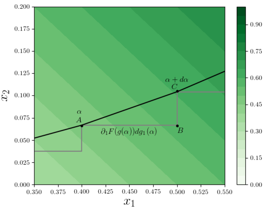
Let's zoom in and look at a specific step $ABC$ in this step-approximation, as shown in figure below:

Path Integrated Gradients

In the above figure, suppose the point $A$ on the path corresponds to path-position $\alpha$ in the parametric path-representation $g$, and $C$ corresponds to $\alpha + d\alpha$ (remember these are infinitesimally-small steps). So the coordinates at $A$ are $g(\alpha)$ and the corresponding function value is $F(g(\alpha))$. As we move along the path from $A$ to $C$, i.e., as $\alpha$ increases by an infinitesimal amount $d\alpha$, the value of the function $F$ changes by a certain amount, and we want to calculate how much the features $x_1$ and $x_2$ contribute to this change. First let's compute the change in $x_1$ when $\alpha$ increases by $d\alpha$. This is given by
$$
dg_1(\alpha) = \frac{ \partial g_1(\alpha) }{\partial \alpha} d\alpha,
$$

and the portion of the function change attributable to this $x_1$ change is $dg_1(\alpha)$ times the gradient of $F$ with respect to dimension 1 at path-position $\alpha$, which is denoted by $\partial_1 F(g(\alpha))$ (we are using the shorthand $\partial_1$ for the partial derivative with respect to dimension 1), and thus the contribution of $x_1$ along this infinitesimal step $d\alpha$ is:
$$
\partial_1 F(g(\alpha)) dg_1(\alpha) \; = \;
\partial_1 F(g(\alpha)) \frac{ \partial g_1(\alpha) }{\partial \alpha} d\alpha
$$

Summing these contributions over all path-positions $\alpha$ yields an integral for the total contribution of feature $x_1$ along the path $\Pi$, and generalizing to any dimension $i$, we can write this definition:

Path Integrated Gradient attribution of function $F$ at $x$, along path $\Pi$, for dimension $i$:
$$
A^{F,\Pi}_i(x) =
\int_0^1 \partial_i F(g(\alpha))
\frac{ \partial g_i(\alpha) }{\partial \alpha} d\alpha.
$$

The reason for the name "Integrated Gradient" should be clear -- we are integrating an expression involving the gradient of the final output of the neural network with respect to the input features. It's important to realize that these gradients are not the same as the gradients used when training the network: the latter are gradients of the loss (which is, roughly, a measure of the "error" between the network output and the desired output) with respect to the network parameters.

As a special case of the above definition, note that the straight line path from the origin to $x$ is given by the parametric representation $g(\alpha) = \alpha x$: as $\alpha$ changes from 0 to 1, we are uniformly scaling all coordinates from the 0-vector until they reach $x$. For this case, note that $g_i(\alpha) = \alpha x_i$ and $\partial g_i(\alpha)/\partial \alpha = x_i$, which implies the following simplified attribution expression, referred to by Sundararajan et. al.^[1:1] as the Integrated Gradient:

Integrated Gradient (IG) Attribution (with baseline = all-zeros vector)
$$
A^{F}_i(x) =
x_i \int_0^1 \partial_i F(\alpha x) d\alpha
$$

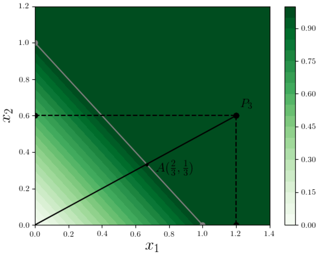
Let's apply the IG method to compute the feature attributions of the function value at $P_3=(1.2, 0.6)$, using the straight line from the origin to $P_3$ in our example where $F(x) = \min(1, x_1 + x_2)$, as shown in the figure below:

At any point on the path from the origin until $A = (2/3, 1/3)$, the sum of the coordinates is at most 1, so the value of $F$ is essentially $x_1 + x_2$, and therefore the gradients $\partial_i F(\alpha x)$ are 1 for both dimensions $i = 1,2$. Between point $A$ and $P_3$, the coordinates add up to at least 1 so $F$ is saturated at 1, and both gradients vanish. The value of $\alpha$ corresponding to point $A$ is $1/(3 \times 0.6) = 1/1.8$. Thus from the above expression, the IG-based contribution of dimension 1 to the function value at $P_3$ is
$$
x_1 \int_0^1 \partial_1 F(\alpha x) d\alpha \;=\; 1.2 \int_0^{\frac{1}{1.8}} 1 \, d\alpha \;=\; \frac{1.2}{1.8} \;=\; \frac{2}{3},
$$
and similarly the attribution to dimension 2 is $0.6/1.8 = 1/3$. Notice how this attribution $(2/3, 1/3)$ is more reasonable than both the attributions we saw earlier using the two extremal paths (see the first figure above):

• the red path gives $(1,0)$; dimension 2 receiving zero attribution is non-sensical, and
• the blue path gives $(0.4, 0.6)$; dimension 2 receiving a larger attribution does not seem "fair" given that $x_1=1.2$ is twice as large as $x_2 = 0.6$.

As mentioned in the previous post, the IG method is the only one among path methods that satisfies all the axioms stated in that post. We should also point out that the integrals in the definitions above are instances of path integrals which have a rich history in Mathematics^[2] and Physics^[3], and in particular Richard Feynman introduced a version of path integrals in his formulation of Quantum Mechanics^[4].

In a future post we will look at other properties of Path Methods and their variants, how the IG attribution can be computed in general, and some simple models where the IG has a closed form analytic expression.